Problems tagged with dimensionality reduction

Problems tagged with "dimensionality reduction"

Problem #058

Tags: pca, projection, quiz-04, dimensionality reduction, lecture-06

Suppose the direction of maximum variance in a centered data set is

\[\vec u = \frac{1}{\sqrt 2}(1, 1)^T \]

Let $\vec x = (2, 4)^T$ be a centered data point.

Reduce $\vec x$ to one dimension by projecting onto the direction of maximum variance. What is the new feature $z$ obtained from this projection?

Solution

$z = 3\sqrt 2$.

The projection onto the direction of maximum variance is given by the dot product with $\vec u$:

\[ z = \vec x \cdot\vec u = (2, 4) \cdot\frac{1}{\sqrt 2}(1, 1) = \frac{2 + 4}{\sqrt 2} = \frac{6}{\sqrt 2} = 3\sqrt 2 \]

Problem #059

Tags: pca, projection, quiz-04, dimensionality reduction, lecture-06

Suppose the direction of maximum variance in a centered data set is

\[\vec u = \left(\frac{2}{3}, \frac{1}{3}, \frac{2}{3}\right)^T \]

Let $\vec x = (2, 1, 2)^T$ be a centered data point.

Reduce $\vec x$ to one dimension by projecting onto the direction of maximum variance. What is the new feature $z$ obtained from this projection?

Solution

$z = 3$.

The projection onto the direction of maximum variance is given by the dot product with $\vec u$:

\[ z = \vec x \cdot\vec u = (2, 1, 2) \cdot\left(\frac{2}{3}, \frac{1}{3}, \frac{2}{3}\right)= \frac{4 + 1 + 4}{3} = 3 \]

Problem #060

Tags: pca, projection, quiz-04, dimensionality reduction, lecture-06

Suppose the direction of maximum variance in a centered data set is

\[\vec u = \frac{1}{2}(1, 1, 1, 1)^T \]

Let $\vec x = (3, 1, -1, 5)^T$ be a centered data point.

Reduce $\vec x$ to one dimension by projecting onto the direction of maximum variance. What is the new feature $z$ obtained from this projection?

Solution

$z = 4$.

The projection onto the direction of maximum variance is given by the dot product with $\vec u$:

\[ z = \vec x \cdot\vec u = (3, 1, -1, 5) \cdot\frac{1}{2}(1, 1, 1, 1) = \frac{3 + 1 - 1 + 5}{2} = 4 \]

Problem #084

Tags: pca, eigenvectors, quiz-04, dimensionality reduction, lecture-06

Suppose $C$ is a $3 \times 3$ sample covariance matrix for a data set $\mathcal X$, and that the top two eigenvectors of $C$ are:

$$\begin{align*}\vec{u}^{(1)}&= \frac{1}{\sqrt2}(-1, 1, 0)^T,\\\vec{u}^{(2)}&= \frac{1}{\sqrt3}( 1, 1, 1)^T, \end{align*}$$

with eigenvalues $\lambda_1 = 10$ and $\lambda_2 = 4$, respectively.

Let $\vec x = (1, 2, 3)^T$ be the coordinates of $\vec x$ with respect to the standard basis. Let $\vec z$ be the result of applying PCA to reduce the dimensionality of $\vec x$ to 2. What is $\vec z$?

Solution

$\vec z = \left(\frac{1}{\sqrt 2}, \frac{6}{\sqrt 3}\right)^T$.

We compute $\vec z$ by projecting $\vec x$ onto each eigenvector:

$$\begin{align*} z_1 &= \vec{u}^{(1)}\cdot\vec x = \frac{1}{\sqrt 2}(-1 + 2 + 0) = \frac{1}{\sqrt 2}\\ z_2 &= \vec{u}^{(2)}\cdot\vec x = \frac{1}{\sqrt 3}(1 + 2 + 3) = \frac{6}{\sqrt 3}\end{align*}$$

Problem #086

Tags: pca, eigenvectors, quiz-04, dimensionality reduction, lecture-06

Suppose $C$ is a $3 \times 3$ sample covariance matrix for a data set $\mathcal X$, and that the top two eigenvectors of $C$ are:

$$\begin{align*}\vec{u}^{(1)}&= \frac{1}{\sqrt6}(-1, 1, 1)^T,\\\vec{u}^{(2)}&= \frac{1}{\sqrt2}( 0, 1, 1)^T, \end{align*}$$

with eigenvalues $\lambda_1 = 5$ and $\lambda_2 = 2$, respectively.

Let $\vec x = (3,2,1)^T$ be the coordinates of $\vec x$ with respect to the standard basis. Let $\vec z$ be the result of applying PCA to reduce the dimensionality of $\vec x$ to 2. What is $\vec z$?

Solution

$\vec z = \left(0, \frac{3}{\sqrt 2}\right)^T$.

We compute $\vec z$ by projecting $\vec x$ onto each eigenvector:

$$\begin{align*} z_1 &= \vec{u}^{(1)}\cdot\vec x = \frac{1}{\sqrt 6}(-3 + 2 + 1) = \frac{0}{\sqrt 6} = 0\\ z_2 &= \vec{u}^{(2)}\cdot\vec x = \frac{1}{\sqrt 2}(0 + 2 + 1) = \frac{3}{\sqrt 2}\end{align*}$$

Problem #090

Tags: lecture-07, quiz-04, dimensionality reduction, pca

Let $\mathcal X_1$ and $\mathcal X_2$ be two data sets containing 100 points each, and let $\mathcal X$ be the combination of the two data sets into a data set of 200 points.

Suppose $\vec x \in\mathcal X_1$ is a point in the first data set. Suppose PCA is performed on $\mathcal X_1$ by itself, reducing each point to one dimension, and that the new representation of $\vec x$ is $z$.

The point $\vec x$ is also in the combined data set, $\mathcal X$. Suppose PCA is performed on the combined data set, $\mathcal X$, reducing each point to one dimension, and that the new representation of $\vec x$ after this PCA is $z'$.

True or False: it is necessarily the case that $z = z'$.

Solution

False.

The principal eigenvector of $\mathcal X_1$ may be different from the principal eigenvector of the combined data set $\mathcal X$. Since $z$ and $z'$ are computed by projecting $\vec x$ onto different eigenvectors, they can be different values.

For example, if $\mathcal X_1$ has maximum variance along the $x$-axis and $\mathcal X_2$ has maximum variance along the $y$-axis, the combined data set might have a different principal direction altogether.

Problem #091

Tags: laplacian eigenmaps, intrinsic dimension, lecture-07, quiz-04, dimensionality reduction

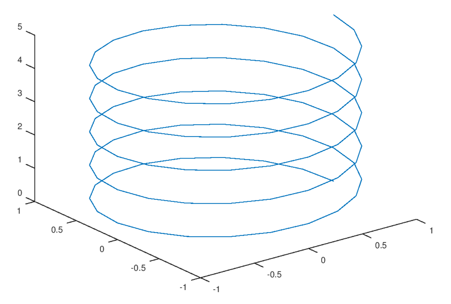
Consider the plot shown below:

Part 1)

What is the ambient dimension?

Solution

The ambient dimension is the dimension of the space in which the data lives. Here, the helix is embedded in 3D space (it has $x$, $y$, and $z$ coordinates), so the ambient dimension is 3.

Part 2)

What is the intrinsic dimension of the curve?

Solution

The intrinsic dimension is the number of parameters needed to describe a point's location on the manifold. For this helix, even though it lives in 3D space, you only need one parameter (e.g., the arc length along the curve, or equivalently, the angle of rotation) to specify any point on it. If you ``unroll'' the helix, it becomes a straight line, which is 1-dimensional. Therefore, the intrinsic dimension is 1.

Problem #092

Tags: laplacian eigenmaps, intrinsic dimension, lecture-07, quiz-04, dimensionality reduction

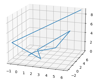
Consider the plot shown below:

Part 1)

What is the ambient dimension?

Solution

The ambient dimension is the dimension of the space in which the data lives. The curve shown is embedded in 3D space (with $x$, $y$, and $z$ axes visible), so the ambient dimension is 3.

Part 2)

What is the intrinsic dimension of the curve?

Solution

The intrinsic dimension is the minimum number of coordinates needed to describe a point's position on the manifold itself. This zigzag path, despite twisting through 3D space, is fundamentally a 1-dimensional curve. You only need a single parameter (such as the distance traveled along the path from a starting point) to uniquely identify any location on it. If you were to ``straighten out'' the path, it would become a line segment, confirming its intrinsic dimension is 1.

Problem #093

Tags: laplacian eigenmaps, dimensionality reduction, quiz-05, lecture-08

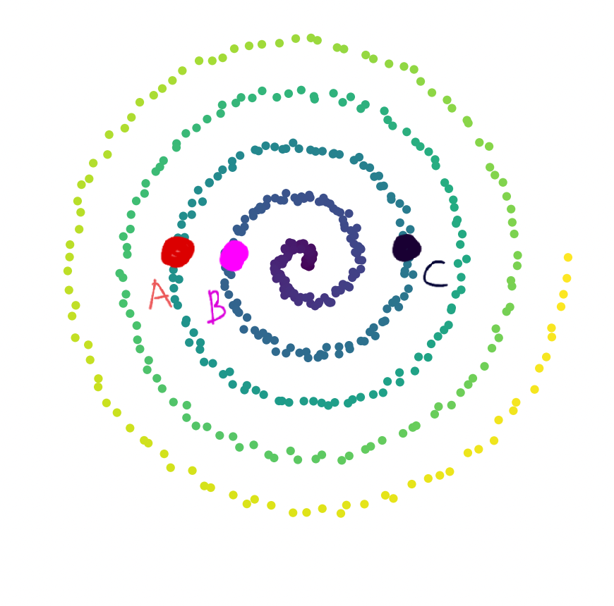
Consider a bunch of data points plotted in $\mathbb{R}^2$ as shown in the image below. We observe that the data lies along a 1-dimensional manifold.

Define $d_{\text{geo}}(\vec x, \vec y)$ as the geodesic distance between two points. Consider 3 points, $A$, $B$, $C$ marked in the image.

Part 1)

True or False: $d_{\text{geo}}(A, B) > d_{\text{geo}}(B, C)$.

True False

Solution

True.

Geodesic distance is the distance along the manifold. If we start walking along the 1-dimensional manifold, starting from the center of the spiral, $B$ comes first, followed by $C$ and $A$. Therefore, $A$ is farther from $B$ than $C$ is from $B$ along the manifold.

Part 2)

True or False: $d_{\text{geo}}(A, C) > d_{\text{geo}}(A, B)$.

True False

Solution

False.

Along the manifold, the order of the points (starting from the center) is $B$, $C$, $A$. Since $C$ is between $B$ and $A$, the geodesic distance from $A$ to $C$ is less than the geodesic distance from $A$ to $B$.